Why it’s vital to model temperature in pipeline simulation
Most density differences along a pipeline are due to pressure, however 10% or 20% of the changes in density are down to temperature.1 This makes temperature an important consideration to build an accurate model for pipeline simulation.
A 10% change in gas temperature linearly affects its density, meaning that in a gas pipeline an isothermal model will not be accurate. Linepack that is calculated without consideration of the temperature differences along the pipeline would be significantly wrong, frictional losses (energy lost in the pipeline) could be 40% off and the flowing gas may be 10% or 20% less dense at the far end of the pipeline than at the inlet.
Extremes of temperature influence the pipeline material too. If metal becomes too cold, it undergoes a brittle transition. This deeply weakens the infrastructure and means that the affected areas must be replaced. Likewise, if a pipeline is warmed too suddenly, it weakens and can become prone to fracture. Temperature also causes the pipeline to expand and contract and this again puts the infrastructure under strain, highlighting the importance of why temperature must be modeled.
This article will look at the key topics surrounding thermal modeling including:
- The heat capacity of a solid or fluid
- The fluid thermal model
- The ground thermal model
- Calibrating the thermal model
The heat capacity of a solid or fluid
Total heat capacity (𝐶) is the energy it takes to raise the temperature of any substance by one unit.1 Most liquids like water behave in a way that their heat capacity’s value is almost the same for a process done at constant pressure (specific isobaric heat capacity 𝑐𝑃) as its value for a process done at constant volume (specific isochoric heat capacity 𝑐𝑉).
For liquids, it is easier to measure isobaric heat capacity than isochoric heat capacity because to keep the volume of a liquid truly constant requires expensive equipment, given the liquid does not fill the entirety of a container. Gas on the other hand is much easier for measuring isochoric heat capacity because it fills any rigid container it is enclosed in.
One advantage of using Atmos Simulation (SIM) Suite is that it calculates all thermodynamic relations for the user. At a given temperature, Atmos SIM will calculate the specific isobaric heat capacity of a pure gas component by assuming that it changes linearly with temperature and interpolating.1 This is a reasonable approximation over the range of temperatures encountered in a pipeline simulator.
The fluid thermal model
The fluid thermal model is solved simultaneously with the hydraulic model.1 During steady state, all heat flows and temperatures are balanced and unchanging over time, however this doesn’t mean that temperature is constant throughout the pipeline.
Temperature in a flowing pipeline is affected by two heat source terms in addition to conductive heat transfer with the surroundings. The terms are:
- Temperature due to friction
- Temperature due to thermodynamic state
The importance of these two source terms depends on whether the pipeline contains a liquid or gas. It also depends on whether the pipeline operates warmer or cooler than its ambient environment.
Heat is typically lost to the ambient environment because it is cooler and friction generates heat as the liquid flows.
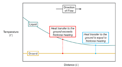
Figure 1: The temperature profile of a flowing liquid (a liquid flows warmer than ambient)
Liquid lines operate at temperatures warmer than ambient and liquid is heated by pump inefficiencies, so it enters warm. Then as it flows along the pipeline, friction turns it into heat and the significant head loss translates energy into frictional heating that is usually affected by pipe diameter.
Looking at the steady profile of a gas pipeline, it enters very hot at the inlet. As the gas flows along the pipeline, pressure drops along the route, which reduces its density.
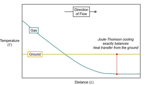
Figure 2: Temperature along a flowing natural gas pipeline settles cooler than ambient
As a gas goes faster further along a pipeline it becomes colder up to a point. Though both are consequences of the reducing density, neither is caused by the other. At lower flow rates, pressure changes less so heat transfer with the environment is more significant and there’s less cooling over a given distance.
The ground thermal model
The ground thermal model starts on the outside of a steel pipeline. The thermal mass of the pipeline wall is treated as if it were part of the fluid in the thermal model, but not convected. This allows for long model time-steps in pipeline simulation while keeping the ground thermal model stable.
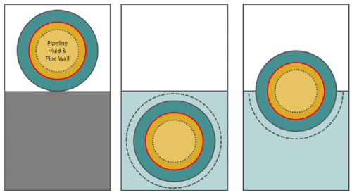
Figure 3: The pipeline wall is at the same temperature as the fluid in thermal model, so any layers beyond the outside of the wall are considered part of the ground thermal model
When the ground thermal model runs, it needs an inner temperature boundary condition at the outer diameter of the pipeline. To do this, it’s coupled with the preceding step’s result from the fluid thermal model. Likewise, when the fluid thermal model is run, it needs the heat transfer at that knot. Results from the preceding steps of the ground thermal model are used to calculate this.
Calibrating the thermal model
Thermal properties are uncertain, which makes calibration of the pipeline simulator very important to make accurate predictions that support the user’s needs. It’s important and good practice to perform a sensitivity analysis to suitably qualify predications around parameters such as soil conductivity and the velocity of the ambient seawater or air. Thermal properties such as this may also vary in line with weather conditions.
If the pipeline simulator is telling us that we’re wasting energy in some way and compressing less vigorously or operating at a lower pressure will solve this, it’s important to first be comfortable trusting the calculations at every unmetered point.
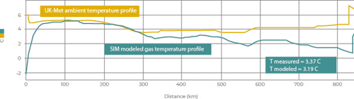
Figure 4: Ambient and pipeline gas temperature profiles modeled in Atmos SIM
The tuning assistant in Atmos SIM helps to automate the iterative manual steps of calibration. This can calibrate thermal parameters, simultaneously recalibrating hydraulic parameters accordingly. This is repeated until the transient time error is within tolerance. It’s been designed to automate offline simulators for controlled refined cases to achieve the correct hydraulic behavior. The tuned thermal and hydraulic parameters can then update the model configuration with one click to accurately predict inventories and arrival times.
References
1 “The Atmos book of pipeline simulation”
Download chapter six Order the book
Ready for chapter seven?
Chapter seven covers how pumps and compressors are a vital component of pipeline infrastructure. Here we look at how pipeline simulation can be used to optimize operations by saving power or with maintenance schedules.