Optimizing a pipeline simulator’s performance
Flaws and uncertainties in pipeline simulation don’t just arise from one specific aspect of the simulator or model but from the overall end-to-end system, including the meters themselves. Sensitivity analysis shows the potential impact of several factors that could generate uncertainty. Addressing the uncertainties that may arise from these factors helps to create a more accurate simulation.
Here we explore how to overcome flaws and uncertainties in pipeline simulations to optimize performance, including:
- The core factors that generate uncertainty
- Troubleshooting when something goes wrong
- Validation and establishing accuracy
The core factors that generate uncertainty
While some uncertainty arises from the simulator, it’s other aspects such as pipeline instrumentation that typically play the major role. There are many factors generating at least some level of uncertainty or error:
- Input measurements - including lags and skews in time
- Pipe parameters - such as wall roughness and inner diameter
- Thermal properties - such as ambient temperature and soil conductivity
- Fluid properties - such as viscosity, heat capacity and density
- Model approach - such as whether to use a transient ground thermal model
- Numerical errors - within calculations of the simulator’s solver
- Empirical correlations - in the model equations such as for friction factor
- The state estimator - interpreting meter data into boundary conditions
- Flaws in the incoming data - in a specific meter, or in data conversion, or in polling1
Any comparison of model versus meter data should bear in mind that meter data is always subject to its own inaccuracies. Every meter is inherently associated with some combination of:
- An offset (also referred to as bias)
- A level of imprecision known as repeatability1
Other factors to be considered include analogue-digital conversion, which introduces an inevitable degree of error or noise in any practical engineering calculation based on field measurements. API 1149 defines the precision of value and its bias with reference to that true value.
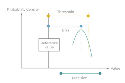
Figure 1: Precision and bias (API 1149), this probability may not be normally distributed if it includes the effects of analogue-to-digital conversion
How important is accuracy in the realms of pipeline simulation?
The purpose of an application, like pipeline simulation dictates its required accuracy, speed and complexity. For example, when batch tracking multi-products, the operating conditions of pressure and temperature are only important for scheduling personnel to the extent that they influence flow rates and flow paths, whereas operations personnel are monitoring if limits are violated.
Similarly, in look-ahead or predictive what-if analysis, the drivers of the simulation are themselves subject to massive uncertainty. The results of the pipeline simulation can only be expected to give a ballpark estimate of future conditions.
It’s important to understand how pipeline simulation handles bad data in online models, where accuracy is regarded as particularly critical.
Troubleshooting when something goes wrong
As previously outlined, how bad data is handled is an important consideration in overcoming uncertainties. Most issues that arise in pipeline simulator accuracy are caused by bad-quality input data being received in real-time from field instruments.
There are loose rules of thumb to troubleshooting issues that may arise during a simulation. For example, if oscillations are observed in the results, they might be due to some combination of the numerical solver and adaptive mesh algorithm.
Validation and establishing accuracy
Rigorous validation is important when establishing the accuracy of a pipeline simulator. Engineers need to confirm that they are getting the correct results, particularly if they will be using the simulator to operate closer to physical or commercial limits. A degree of inaccuracy is always present in any model, our task is to ensure it’s always within acceptable levels. This ensures that pipeline operations proceed smoothly while meeting professional and legal requirements.
There are different ways of validating a model. We may compare simulated results against analytical results or measured values or we may reasonably subject the model to any of the following tests:1
- Analytical solutions for special cases of shut-in, steady state, or transients
- Numerical approximations manually confirmed using spreadsheets
- Common sense ballpark figures, reasonable profiles, mass balances
- Solving again in the same pipeline simulator with a more refined mesh
- Solving independently using different vendors’ software packages
- Field tests using historic datasets to verify what happens on site
Comparing simulated results against analytical results
Many manual calculations are easy enough that engineers refer to them as back-of-the-envelope. Such calculations are typically steady state, but one valuable example of a straightforward calculation validating a transient operation is the Joukowsky equation. Analytical results are one way we use to determine the accuracy of a pipeline simulator’s results. In the case of Joukowsky’s equation, it validates fast-transient surge events in isothermal conditions.
Acceptance tests and historic datasets
Once internal checks have been made in the model, real process data is leveraged to build confidence in the model by verifying model calculations on site.
Every project has key milestones including a factory acceptance test (FAT), an integration factory acceptance test (IFAT) and a site acceptance test (SAT). These may take place years apart if a pipeline is under construction, which presents a challenge for project delivery as well as for data logging and validation. Some projects have a model acceptance test (MAT) inspecting the model in isolation.
Gas pipeline operators rely on real-time models to estimate the inventory held as linepack, so it’s crucial they have confidence in their model. There are a few ways to validate against historic data. When assessing how well a pipeline simulator performs on site, we are asking several questions at once, including:
- Can we accurately deduce the value of a missing meter that it does not know about?
- What is the overall impact of a particularly uncertain model parameter (eg thermal model)?
- Can the overall end-to-end system handle periods of bad meter data effectively?1
It’s the accuracy of a model which allows us to then ask questions concerning further results such as:
- Does an unmetered offtake trigger a leak alarm during all kinds of operations and in shut-in?
- Does the leak detection system provide an accurate estimate of leak flow rate and location?
- Does the estimated arrival time (ETA) of a scraper or a composition peak agree with reality?
Once the site data becomes available, there is an initial period of site validation, adjusting model parameters, recalibrating and setting the automatic tuning (learning) to update itself continuously.
Overcoming uncertainties in pipeline simulation
Implementing simulation systems provides pipeline operators with the ability to answer many questions and assist with day-to-day tasks. However, it’s crucial to maintain a proper process for rollout to help reduce the uncertainty of implementing the system.
Using validation techniques like comparing simulated results against analytical results and subjecting the model to reasonable tests help to establish accuracy.
References
1 “The Atmos book of pipeline simulation”
Download chapter three Order the book
Ready for chapter four?
Chapter four covers a range of equations of state that can be used to express thermodynamic properties dependent on two others and the particulars when considering these calculations for pipeline simulation.