Steady states in a pipeline
In hydraulics, a steady state is a physically stable way to operate a pipeline.
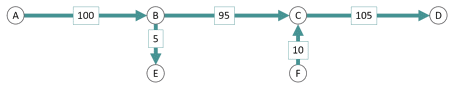
Figure 1: A pipeline in a steady state: flows are perfectly balanced, unchanging over time
Pipeline operators give due consideration to steady state operating conditions because they are a useful way of looking at what a pipeline does, though they do not represent the most challenging pressures seen by their pipeline (associated with transients). To model the steady state hydraulics of a liquid pipeline we can take advantage of some simplified physics. When we apply a similar approach to steady states in a gas pipeline, we find the varying density adds some complexity.
When in steady state, flows of mass (𝑀), momentum (𝑀∙𝑣) and energy (𝐸) are all in perfect balance, unchanging over time. The mass flow rate, usually expressed as an equivalent volumetric flow rate, is driven by a special sort of mechanical energy associated with a fluid, known as its hydraulic head. A fluid flowing along a pipeline incurs head loss, due to several effects which are lumped into the concept of friction. The frictional effect may depend on factors such as the roughness of the pipe wall, and fluid’s density and viscosity.1
When it comes to modeling, steady state models are easier to implement than a transient model. The calculations are sometimes simple enough that they can be done in a spreadsheet, allowing the user of a pipeline simulator to do a basic reality check to ensure the steady state is giving expected results. Steady states are essential for simulating gas and liquid pipelines.
For example, to commence a transient scenario, we need to first “cold-start” by solving a steady state prior to progressing subsequent steps. Moreover, there are a number of applications in which steady states are as useful as transient scenarios, or indeed more useful, facilitating flow assurance throughout the pipeline lifecycle.
In this article we will look at a few key aspects of steady states, and how a user can calibrate them in pipeline simulation to improve the performance of their model. We will cover:
- Steady hydraulics in liquid pipelines
- Steady hydraulics of gas pipelines
- Calibration of parameters using steady states
Steady hydraulics in liquid pipelines
Any pipeline is subject to reasonable limits on flow velocity. Typically, this is 1 or 2 m/s in a liquid line, where a velocity beyond that limit could incur unacceptable frictional losses or cause severe erosion.1 To achieve a desired flow rate while making flow velocity more tolerable, a designer could select a larger diameter pipeline or add a “loop-line” in parallel to an existing mainline. This kind of decision making involves weighing up the capital and operating costs of each possible approach against other options. A pipeline simulator allows many scenarios and configurations to be conveniently compared making it a great tool for offline studies.
Some locations in a liquid pipeline are prone to over-pressure which means that maximum allowable operating pressure (MAOP) could be exceeded, violating an acceptable limit on operating conditions. If the over-pressure violation is too severe, there is a risk that the pipeline may weaken or burst. Conversely, some locations are prone to falling below the lowest allowable operating pressure (LAOP). This limit may be in place to keep the operating conditions above the liquid’s vapor pressure, so if a pipeline drops below the LAOP anywhere along its route, a vapor bubbles could form.
Operators refer to this as column separation or slack-line and if the bubbles collapse in an unplanned way they carry a risk of creating shockwaves in the pipeline. Over time this kind of event may cause fatigue in the pipeline by erosion and corrosion, ultimately leading to a potential rupture. Both maximum and lowest allowable operating pressure (MAOP and LAOP) are set conservatively, applying reasonable margins to stringent safe operating limits (SOL). It is excursions beyond that safe limit which pose a safety hazard, rather than “merely” a risk of disrupting routine operations.
Although real pipelines have varying elevation, diameters and liquid properties, it is insightful to start thinking of steady states by considering the hydraulics of a flat liquid pipeline. We can make a few important statements about this special case, a flat liquid pipeline flowing at a steady state:1
- In the laminar flow regime, pressure drop is proportional to flow rate
- In the turbulent flow regime, pressure drop is roughly proportional to flow squared
A pipeline simulator, like Atmos Simulation (SIM) Suite, can calculate how the pressure and head varies throughout a liquid pipeline using a hydraulic profiler.
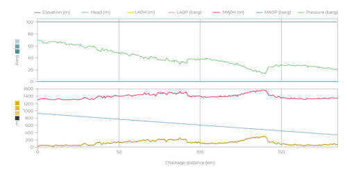
Figure 2: A hydraulic profiler in Atmos SIM shows that pressures remain within the limits of MAOP and LAOP along the entire length of this liquid pipeline
If transporting heavy hydrocarbons such as crude oil, the operator might inject additives known as drag reduction agents (DRAs) to make the properties of these fluids more amenable to pipelining. Since DRAs affect the flow behavior of the commodity, controllers require their simulator to not only capture the effect of DRA but also configure, solve and analyze countless scenarios in order to ascertain how much DRA is optimal and at which locations to inject it along the pipeline. This is one application in which the steady hydraulics of liquids are intertwined with the physics of more complex problem-solving for pipelines.
Steady hydraulics of gas pipelines
Gas pipelines are typically operated in a condition of imbalance, rarely if ever reaching a steady state. Instead, a given section of a gas pipeline is packing (gaining inventory) or unpacking (losing inventory), a process known as linepack.1 Nonetheless, nominal steady states let us define the operating envelope of a gas pipeline, the maximum and minimum flow rate which can be maintained indefinitely, giving us an excellent place to start when analyzing the hydraulics of a gas pipeline.
If we consider a steady state with the same flow rate all along a gas pipeline, we find that unlike in a liquid pipeline, flow velocity is not constant along the route. Indeed, the flow velocity always varies as a profile along a gas pipeline, even in a steady state.
If it seems surprising that the same flow rate corresponds to different velocities at different distances along the route, consider the definition of a gas. A gas is compressible, the density changes depending on the pressure. The pressure is different at different points along a pipeline, therefore gas velocity must vary, even in a fixed diameter pipeline carrying the same flow rate everywhere in a steady state. This fact makes various simple questions surprisingly difficult to answer without a pipeline simulator, even in a steady state.
For example, how long does it take for a pig to travel the length of a gas pipeline? It will get progressively faster along its way. The maximum allowable flow velocity in a typical gas pipeline is usually 5 to 12 m/s for a typical natural gas. Beyond 15 m/s carbon dioxide (CO2) corrosion becomes an issue and any faster than 18 m/s the noise becomes unacceptable. Atmos SIM can alert the user if the velocity approaches these limits at any point along the pipeline.
Gas pipelines must remain within MAOPs and LAOPs just as liquid lines. The MAOP along a gas transmission pipeline is typically well above 100 atmospheres. In practice, a gas transmission pipeline is operated to maintain a minimum allowable linepack corresponding to a shut-in LAOP. This is different to the LAOP during a flowing operation.
A LAOP may be contractually specified at the demand points reaching each customer. Depending on the elevation profile along a gas pipeline, the pressure may fall well below the delivery pressure at some point along its route. A simulator can alert the user of any violation of LAOP anywhere in the gas network, monitoring the entire length of the pipeline to help ensure operating pressure never falls too low.
Both the MAOP and LAOP are set cautiously, with responsible engineers applying stringent margins that guarantee the real operation adheres to regulations and guarantees safe operating conditions. These limits of MAOP and LAOP, together with the performance constraints of equipment such as compressors, are what define the feasible steady states bounding the operating envelope of a gas pipeline.
An important consideration intertwined with the hydraulics of gas pipelines is temperature limits. A gas pipeline can get so cold that there is a risk of freezing if left unchecked, just as with pressure, careful measures are taken to control temperature through operations planning. If liquid is present anywhere along a freezing pipeline it may turn to ice, resulting in blockages especially in valves.1
Since gas is compressible, its density changes as a function of pressure and temperature. Conservation of mass applies in a simplified form in a steady state, known as a mass balance. The pipeline industry expresses mass flow rate in a slightly different way: standard volumetric flow rate, often referred to as “standard flow”. Atmos SIM demonstrates the consequences of conservation of mass when we set up any scenario involving the blending of incoming gas flows with different compositions, such as blending rich gas with lean gas, or blending hydrogen into natural gas.
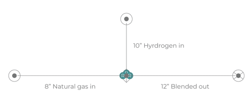
Figure 3: Blending incoming flows of natural gas with hydrogen in Atmos SIM
Calibration of parameters using steady state
The state of a real gas pipeline is never truly steady, but we can deduce an equivalent steady state to calibrate the parameters of our model. This is essential for a pipeline simulator such as Atmos SIM to give accurate results representative of the real pipeline. To deduce an equivalent steady state, the first step is to identify a stable operation in the historic dataset which continues long enough that it spans the pipeline’s throughput time. During this period, the pipeline was operated in such a way that we expect any transients to have actually settled to something resembling a steady state. We then take an average of these stable conditions over that time-scale.1 Finally the average flows and pressures form the basis for hydraulic calibration, to align uncertain model parameters such as wall roughness. This makes the model accurately predict the flow rate at different pressure drops.
Several tuning cases are performed in a pipeline simulator before it is considered well-calibrated. Although the pipeline simulator should initially give good approximate results, there is always a phase for fine-tuning during a simulation project which makes the model much more accurate. Atmos SIM makes this process easier by automatically finding suitable values to calibrate the model using a feature known as the tuning assistant.
This feature solves a steady state with an initial guess for the parameter being calibrated, automatically analyzes the results, improves its guess, and solves again. In this way, Atmos SIM calibrates the wall roughness, overall efficiency, and inner diameter of the pipeline to match flow, pressure drop and arrival time.
This can be done automatically in tandem with the calibration of thermal parameters to ensure accurate temperature along the line, including overall heat transfer coefficient, ground thermal conductivity, burial depth and velocity of ambient medium.1 The tuning assistant empowers the engineer with one-click tuning of any pipeline property, for expedient calibration of accurate models.
Steady states help professionals design and operate pipelines
Although Atmos SIM offers an advanced physics engine capable of handling fully transient pipeline simulation, it also takes full advantage of steady states in their proper scope of application, serving the needs of designers, planners and control room operators of gas and liquid pipelines. The steady state as a fundamental concept and practical engineering principle helps a user understand how fluids flow through pipelines, validate the results of their simulation and calibrate their model parameters.
References
1 “The Atmos book of pipeline simulation”
Download chapter six Order the book
Ready for chapter six?
In chapter six we look at the importance of thermal modeling in pipeline simulation. From how temperature affects the pipeline to how Atmos Simulation (SIM) Suite can help with calibration.